
A new online ultrasonics components store has just opened at www.UltrasonicsWorld.com. Check their amazing prices for replacement ultrasonics components, fully compatible with the major manufacturers' originals at a fraction of the cost.
You are here
Chapter 6 - Measurements - Dies and Mountings
Design and optimisation of an ultrasonic die system for forming metal cans
6. MEASUREMENTS - DIES AND MOUNTINGS
6.1 EVALUATION OF MODE AND FREQUENCY
6.1.1 Physical methods for evaluating mode of vibration
6.1.2 Admittance / Impedance Plotter
6.2 RESULTS OF MEASUREMENTS ON ULTRASONIC DIES
6.2.1 Mode evaluation using talc
6.2.2 Admittance plotter measurements
6.2.2.1 Admittance plotter measurements - transducers
6.2.2.2 Admittance plotter measurements - die tuning
6.2.2.3 Admittance plotter measurements - dies and mountings
6.2.2.4 Admittance plotter measurements - mounting evaluation
6.2.3 Comparison with FE predictions
6.2.4 Accuracy of FE predictions
6.3 ESPI MEASUREMENTS
6.3.1 Principles of ESPI
6.3.2 Converting FE results to simulated ESPI plots
6.3.2.1 Pure modes
6.3.2.2 Distorted modes
6.3.3 Comparison of results
6.3.4 ESPI Summary
6.4 EVALUATION OF TUBULAR MOUNTING PERFORMANCE
6.4.1 Free vibrations of steel prototype
6.4.2 Admittance plotter measurements of mounting performance
6.4.3 Tubular mounting measurements - summary
6.5 MEASURED PROCESS FORCES
6.5.1 Evaluation of forming force in early work
6.5.2 Evaluation of forming force in later work
6.6 CONCLUSIONS
MEASUREMENTS - DIES & MOUNTINGS
The die design work described in the previous chapters has been largely theoretical. This was backed up by practical verification at the time, to ensure the validity of the theoretical models. Some of this verification work was by comparison with other theoretical models, and this was described in chapter 3. The work described here is the ultimate verification - the physical testing of dies manufactured for various processes during the course of the project.
For the ultrasonic dies and mountings designed by finite element analysis the essential verification involved simple checks on the performance and the longevity of a component. More detailed testing was also used to help estimate the likely accuracy of future finite element models.
The purpose of this chapter is to describe methods of testing the ultrasonic equipment, to record the measurements made and to compare the measurements where possible with the theoretical expectations.
6.1 EVALUATION OF MODE AND FREQUENCY
Electronic equipment for the measurement of frequency is readily available. This can be used to measure the driving frequency of the power supply to the die, but to be meaningful this information must be related to the response of the die.
The simplest method of evaluating vibrations is using a power meter to monitor the electrical power being supplied to the transducer. Provided that the high frequency power supply operates at (approximately) constant voltage the input power will peak at resonance. Voltage is effectively equivalent to force, and current to amplitude. This is a useful method of finding a resonance but gives no information on the mode of vibration.
There are several 'traditional' physical methods for determining the die's motion as illustrated in figure 6.01. The relevant ones will be described in turn.
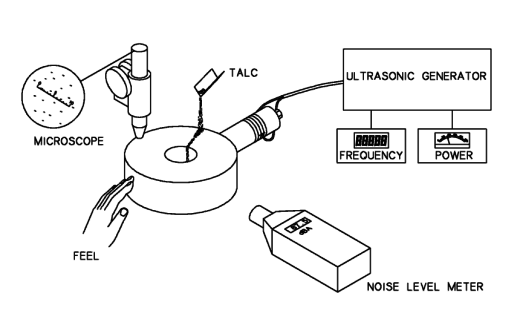
Figure 6.01 - "Traditional" methods of measuring die vibration
6.1.1 Physical methods for evaluating mode of vibration
One simple and sensitive method of testing the vibrations is the 'feel' of the die surface - activity can be gauged roughly by gently touching the vibrating surface. High amplitude vibration is indicated by an oily, frictionless feel. Note that this technique is not generally recommended because of possible medical effects which may include tissue damage due to vibrations and / or burns from energy transfer. Ultrasonics are used in physiotherapy but at higher frequency and much lower power. Some of the physical / safety effects of ultrasonics are discussed in section 1.4.
Another physical output of most ultrasonic systems which also has obvious safety implications is the airborne noise. Using a sound level meter at a fixed distance this can be used as a measure of die activity. By moving the meter around the die at a fixed distance it is possible, in theory, to find areas of high and low activity. In practise, however, picking out different modes of vibration by this method is very difficult because of the radiation of noise in all directions from all parts of the die.
Use of a sound level meter will also show whether the operator is at risk from the noise emitted - hearing protection should be worn if the operator is to be close to unshielded equipment for a significant time. Again, see section 1.4 for a discussion of the safety aspects of ultrasonic noise.
A simple, non-hazardous method of indicating the mode of vibration is using fine powder (talc). The die must be set up with its axis vertical and while it is vibrating in some unknown mode the talc is sprinkled on the flat top face. The vibrations cause the talc to move over the surface and each mode of vibration shows a characteristic pattern of talc flow. The use of this technique to evaluate vibrations of circular plates (producing "Chladni figures") was described by Waller [113]. For example, if the die was working properly in the R0 mode (as described in chapter 3) then the talc would flow smoothly inwards to the hole in the centre, whereas if the die was vibrating in the R3 mode there would be six areas (corresponding to the nodal points) where the talc would not move or would move tangentially. Figure 6.02 shows some talc patterns observed, and these are discussed in section 6.2.1.
A more sophisticated method used for measuring the amplitude on the outside surface of the die was the Telsonic amplitude meter. This device uses an eddy-current sensor for sensitive measurement of distance and electronic processing to produce a digital readout of amplitude perpendicular to the surface. No special mounting is required - the probe is simply held close to the vibrating surface. The measurements depend on the electrical properties of the material so the system is only applicable to aluminium and titanium (the materials for which it was calibrated). Because of its high purchase price this piece of equipment was obtained only on hire to evaluate the motion of a specific die when required. See the work of Chapman and Lucas [114, 115] for some results obtained from this equipment and used in modal analysis.
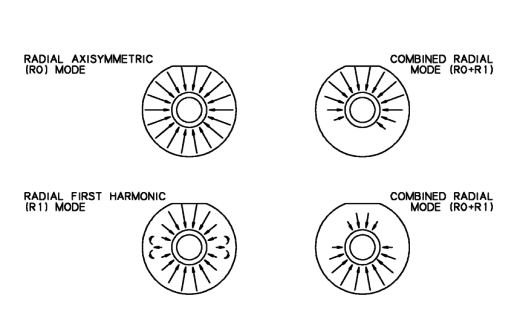
Figure 6.02 - Patterns of talc movement
All of the methods described above were used in early work on ultrasonics at CarnaudMetalbox. The high frequency power supply used at that time offered full manual control of frequency. This allowed the user to drive the ultrasonic tooling over a wide range of frequencies and determine its response, using a power meter and by physical methods. For later work, however, ultrasonic systems from the plastic welding industry were used. The single-frequency dedicated ultrasonic generator and transducer were capable of operating at much higher efficiency than the earlier system (and hence providing greater amplitude) but were not suitable for operating over a wide frequency range. Furthermore the operating frequency is not under the control of the operator, instead an automatic frequency control 'latches on' to resonance. These systems are therefore not suitable for full testing of the ultrasonic tooling. Appendix 7 contains specifications for the ultrasonic generators and transducers used in this work.
6.1.2 Admittance / Impedance Plotter
Following the adoption of single-frequency ultrasonic systems there was a need for a dedicated test system to perform the measuring functions which the new equipment could not handle. The equipment selected (called an Admittance / Impedance Plotter and supplied by Sonic Systems [116]) comprises a variable frequency generator with output voltage suitable for piezo-electric transducers. A digital frequency meter gives an accurate measure of the output frequency, which can be adjusted manually or set to scan automatically over a range at variable scan rates (for specifications see Appendix 7).
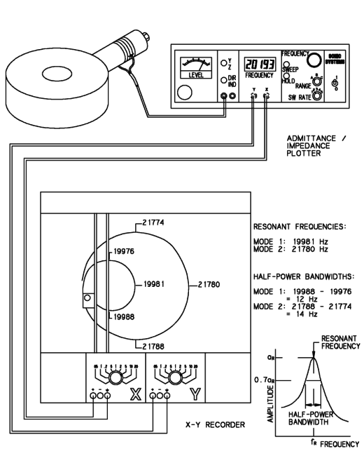
Figure 6.03 - Measurements using Admittance Plotter
The most useful feature however is the signal output of the electrical admittance (or impedance) of the transducer. Two signals are provided, corresponding to the real and imaginary parts of the admittance / impedance and these should be connected to the X and Y inputs of a chart recorder. Thus the complex admittance or impedance is displayed as a point on a polar plot (a conventional form of display for complex numbers) and the variation with frequency is displayed as a curve.
This is useful because over a wide frequency range (eg 16 to 24 kHz) the electrical properties of the ultrasonic transducer change only gradually. The observed variation in electrical admittance or impedance depends almost entirely on the mechanical resonances of the transducer and anything attached to it. As the frequency is scanned through a resonance the admittance plot describes a circle, while scanning through an antiresonance causes the impedance plot to describe a circle.
Of these, the admittance plot is generally the more useful. It can be shown [68], [116] that the point of zero imaginary admittance corresponds to resonance while the points of minimum and maximum imaginary admittance (at 90° on the circle) correspond to the half-power points. Furthermore the size of the circle is inversely proportional to the power losses in the system. (Note however that this information should be treated with caution - this is an indication of power loss at low amplitude but material damping can be very non-linear so results at high amplitude may not correspond.) Figure 6.03 shows the general arrangement of equipment and a typical circle plot with the significant features marked for clarity.
By careful study of the admittance plot and the frequency meter the following information can be obtained for each resonance:
Resonant frequency
Half power bandwidth
'Q' factor
System losses
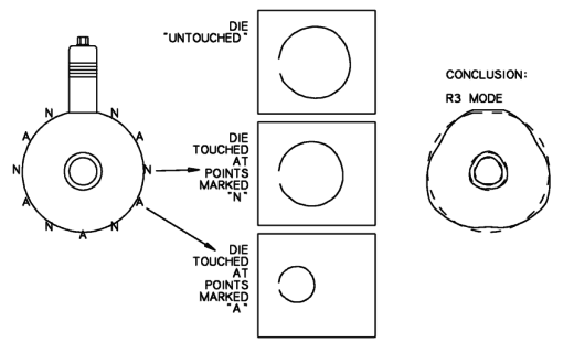
Figure 6.04 - Mode identification using Admittance Circle Plotter
With a little further effort the user can also gain a clear idea of the mode of vibration. The generator frequency should be set to resonance with the pen plotter (or a simple voltmeter) indicating the real component of admittance. When the die is touched the extra losses introduced by a human finger are detectable by a reduction in admittance (the circle becomes smaller). The safety concerns about touching vibrating tools described in the previous section are not relevant here because the power output of this generator is very much smaller. The reduction in admittance depends on the mode of vibration and where the die is touched. Touching at a vibration node will have little or no effect on the admittance while touching at an antinode will have most effect. Thus by touching the die and watching the admittance display the user can quickly identify nodal areas (if any) and hence establish the mode of vibration. Figure 6.04 demonstrates the principles of this method.
6.2 RESULTS OF MEASUREMENTS ON ULTRASONIC DIES
6.2.1 Mode evaluation using talc
Figure 6.02 shows some typical talc patterns found in early work on this project. In these diagrams the arrows show the direction of the observed talc flow and the relative size of the arrows indicates roughly the speed of flow.
Note that while the relative amplitude of different areas of the die is clearly shown (by the size of the arrows) all phase information is lost. In both the radial axisymmetric (R0) and the radial first harmonic (R1) mode the areas at the top and bottom of the die (in this view) appear identical. The arrows indicate that for both modes the talc moves quickly towards the centre of the die. The important difference is that in the R0 mode these areas are in phase, moving inwards and outwards together, whereas in the R1 mode they are 180° out of phase ie. the top moves inwards while the bottom moves outwards. (See section 3.1 for a detailed description of these modes.) It is this phase difference which accounts for the cancellation of amplitude over a part of the die which is seen in the combination modes. Depending on the phase angle between the R0 and R1 modes and their relative amplitude, cancellation of movement can occur at either top or bottom of the die or anywhere in between, while in other areas the movement due to the two modes will add to give increased motion.
At the time these measurements were made the unwanted harmonic modes of vibration were not understood and the uneven modes of vibration were blamed (wrongly) on a poor interference fit between the inner and outer parts of the die.
6.2.2 Admittance plotter measurements
In later work finite element analysis was used to help in understanding the unwanted modes of vibration and in predicting their natural frequencies. The admittance plotter measurements were so complete and accurate that most work in evaluating the performance of ultrasonic dies was done using this method. Tables 6.01 to 6.05 and 6.12 to 6.13 show many of the results obtained. In each case the resonant frequency, half-power bandwidth and circle diameter (in mV) is recorded for each resonance, along with any other relevant measurements obtained (eg. power input at a given amplitude level). Note that power and amplitude measurements must be treated as approximate indications because of unknown calibration of the various meters, although comparisons should be valid between measurements using the same ultrasonic equipment.
The measurements taken, and the corresponding descriptions / comments have been divided into four categories: transducers, die tuning and miscellaneous dies and mountings are included here. Use of the admittance plotter in evaluating the mounting is described in section 6.4.2.
6.2.2.1 Admittance plotter measurements - transducers
Table 6.01 shows measurements of various transducer systems used for this work (see appendix 7 for equipment details).
Items 1 to 7 are all measurements of the same component (the Kerry Ultrasonics transducer serial number 757). Multiple measurements were made because a circle plot of the transducer alone was usually made as a reference at the beginning of each series of tests (eg tuning a die). This shows some variability in the measurements. The transducer varies in frequency from 19911 to 20035 Hz and in circle diameter from 56 to 63 mV. The measurements were made with the transducer resting on a flat surface (eg a table or bench) so the changes in circle diameter (indicating changes in power losses from the component) could be caused by differences in its positioning or in the coefficient of friction on the surface. This would not account for the changes in resonant frequency, however. Some variability would be expected as a result of temperature variations but there is also a general trend of frequency rising with age. This might be caused by gradual aging of the piezo-ceramic crystals or by "bedding in" of the interfaces. In any case the rate of frequency rise is not great enough to cause any problems.
Items 8 and 9 are measurements of the second Kerry transducer, serial number 786, which was apparently identical to the first. These show a slightly higher resonant frequency and a smaller circle diameter (average 51 mV compared to 60 mV). This indicates a slightly greater power loss from the second transducer. The greater half-power bandwidth of transducer 786 (34 Hz compared to 27 Hz average) also indicates higher power losses. Note that the half-power bandwidth can only be used to compare power losses in this case because the two components are nominally identical. At constant frequency the power loss is proportional to half-power bandwidth and to stored energy. The stored energy is a function of size, shape and material so it should be the same for two identical transducers.
Item 10 is another transducer from a different manufacturer (Telsonic Ultrasonics) which also features an integral "can" to guard the electrical connections to the transducer (useful because high voltages are used) and also to protect the transducer from damage due to accidental knocks. Despite this extra component which must absorb some power, the large circle diameter indicates lower power losses than for either of the other transducers. In fact this transducer is made from aluminium alloy, whereas the others are made from titanium alloy and steel. The moving mass of the Telsonic transducer is therefore less than that of the Kerry transducers and hence its stored energy is less. It is this that allows the Telsonic transducer to operate with lower power losses. The difference in stored energy could also be deduced from consideration of the half-power bandwidth of the Telsonic transducer - it has a larger half-power bandwidth (49 Hz compared to 34 or 27 Hz) but a smaller power loss (indicated by the circle diameter) so its stored energy must be less.
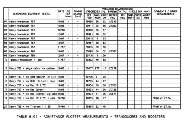
Item 12 shows the result of fixing the Kerry transducer (number 786) to the magnetostrictive transducer system used for the early work on this project. This result is remarkable for the huge half-power bandwidth and the tiny circle diameter which indicates very high power losses. The inefficiency of the magnetostrictive system in comparison with the piezo-electric ones has also been demonstrated by direct measurement of power and amplitude so this type of result is to be expected. Note also that the large half-power bandwidth has a positive benefit in allowing the transducer to operate over a wide frequency range, as discussed in section 1.1.5.
Items 14 to 21 show the results of fitting various interstage horns ("boosters") to the Kerry transducers. The aim was usually to give a reduction in amplitude because the transducer was vibrating at approx 27 μ whereas the die design indicated a limit of 20 μ. Measurements with the booster alone (items 14,16,21) show a slight reduction in circle diameter, indicating a small increase in the power loss. The other reason for using a booster was to fit a guard (case) around the transducer. This was fixed to a nodal flange on the booster so that (theoretically) no energy would be transmitted from the vibrating system to the case. In practise the measurements indicate a further increase in the power loss and the system with booster and case had a circle diameter about half that of the transducer alone (ie twice the power loss). Measurements were also made of the power and amplitude (using the meters on the Kerry system). Reference to these and the circle diameters suggests that approx 150 W is required to operate the Kerry transducer at 27+ μ, with a further 150 W lost in the case, if fitted.
One further comparison is also shown in this series of measurements (items 17 and 18). A system comprising transducer, booster and case was measured with the Admittance plotter connected directly to the transducer, and connected via a cable 3 m long (this cable was used to supply the transducer while it was used for can necking in the hydraulic press). The direct / indirect switch on the admittance plotter was also changed accordingly. There was no significant difference between the readings, indicating that the use of the extra cable did not impair the performance of the ultrasonics.
6.2.2.2 Admittance plotter measurements - die tuning
Tables 6.02 to 6.04 show the tuning procedure for six ultrasonic dies. The method of tuning a new die is described in detail in section 3.8, but the essential point is that the die must be manufactured oversize on outside diameter and gradually machined down until the resonant frequency meets the requirement (usually 20 ± 0.1 kHz).
Items 1 to 7 in table 6.02 show the tuning of a die constructed from a titanium alloy outer with a ferro-titanit insert, used for necking a 45 mm diameter aerosol can to 33 mm diameter. Note that for this system (die and transducer) three resonances have been found at each stage of the tuning process. By widening the frequency range many more resonances could have been found for all systems tested. In general only those in the range 18 to 22 kHz have been noted because outside this range the other resonances have not been found to cause a problem.
For the initial measurement of the die as manufactured resonant frequencies were found at 18.1, 19.6 and 21.5 kHz. From the finite element analysis it was expected that the R1 (first harmonic) would appear below the R0 (axisymmetric) and the R3 (third harmonic) above it. It was therefore expected that the three resonant frequencies corresponded to R1, R0 and R3 modes respectively. Touching the die and noting the response of the admittance plotter (as described in section 6.1.2) confirmed this. In general the resonant frequencies have been recorded with the R0 frequency first, followed by the unwanted resonances.
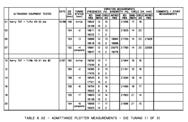
As manufactured the R0 frequency was too low. This is normal because the die is made oversize with an allowance for tuning. During tuning the outside diameter of the die was progressively machined down, in this case from 156 mm diameter to 154, 153 and finally 152 mm. As a result the R0 frequency increased towards 20 kHz and the tuning process stopped when the frequency was 19.98 kHz (well within the specified limits). The relationship between frequency and diameter is fairly linear, as shown in figure 6.05. Typically the frequency rises by about 90 Hz per 1 mm reduction in diameter.
Note that during the tuning process both the R1 and R3 frequencies also rise. This is the reason why, in general, the problems experienced with interference from the unwanted harmonic frequencies cannot be solved by a change in the working frequency.
Note also that the circle diameter increased slightly as the tuning progressed. There are two likely reasons for this. Firstly as metal is removed from the die there is less moving mass and hence less energy loss. Secondly when the resonant frequency of the system is low there is a significant mismatch between the frequencies of the die and the transducer. Since the transducer is forced to operate away from its resonant frequency the interface between the die and transducer is not at an antinode (a stress node). This gives rise to power losses from friction at the interface.
Items 10 to 20 are the measurements made while tuning a similar die for necking a 45 mm aerosol can to 31 mm diameter. The die is again constructed from a titanium alloy outer with a ferro-titanit insert. The tuning is similar and the comments above apply equally well to this die also. The final die diameter achieved is 2 mm greater than the earlier die, probably because the inside diameter is smaller in this case.
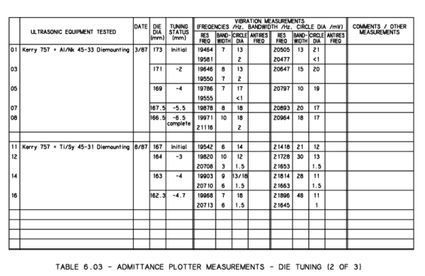
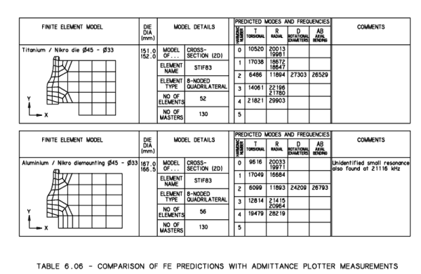
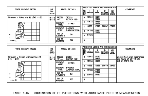
In table 6.03 items 1 to 6 are the measurements made while tuning another die for necking 45 mm aerosol cans to 33 mm diameter. In this case a ferro-titanit insert has been fitted in an aluminium "diemounting" (combined die and tubular mounting in one piece). Note that the tuned diameter (166.5 mm) is considerably larger than the earlier die (152 mm). This was predicted by the finite element analysis (and could also have been predicted by the design graphs of chapter 4 and appendix 5), so the initial, as manufactured, diameter of the die was increased accordingly.
The power loss for this die (as indicated by the circle diameter) is comparable, or slightly better than, the earlier dies. Aluminium is inherently a less "lossy" material but extra losses were introduced by the mounting tube and these effects approximately cancel. This is a good result for the mounting, indicating a relatively small power loss. Mounting performance is discussed further in section 6.4 and results are given in tables 6.12 and 6.13.
Note how close the unwanted harmonic frequency appears in this die (20.964 kHz after tuning). This is the third harmonic (R3) frequency which for the two earlier dies appeared at about 21.7 kHz. This is a particular problem for this combination of materials and geometry, leading to "mode switching" in use (see section 3.3.2). In this case the problem can be avoided by simply using other combinations of materials as shown by the results for the other die in table 6.03 and both dies in table 6.02.
Items 11 to 16 in table 6.03 show the results for another die, in this case constructed from a titanium alloy diemounting with a Syalon insert (see section 3.7 for a detailed description of the materials used for these dies). This again shows a relatively large circle diameter (provided the die was held at the mounting flange not placed on its face) and the R3 frequency at 21.9 kHz is separated from the working frequency far enough to avoid mode switching. Two new circles have also appeared at 20.7 and 21.6 kHz but these are very small (1.5 and 1 mV respectively) and so would not be expected to cause any problems. These are probably resonances of the mounting tube, remnants of the multiple resonant frequencies of the free mounting. Some tiny circles were often found in the circle plots of dies with mountings but circles of diameter less than 1 mV were generally not recorded.
Table 6.04 shows the results recorded while tuning two "shaped dies" (for further details see section 3.6). Items 1 to 9 are for a die made from aluminium alloy with a ferro-titanit insert with a profile suitable for necking 45 mm aerosol cans to 31 mm diameter. This is very similar to the diemounting (items 1 to 8 of table 6.03) which showed problems with the closeness of the R3 frequency. In fact this was deliberate. Knowing the problems with this combination of materials and geometry this die was constructed specifically for the purpose of testing a theoretical solution - the three-flat shaped die.
The initial results were recorded for the die before the three-flat shape was machined onto it. This shows the R0 and R3 frequencies where they would be expected (the R0 lower than 20 kHz before tuning, the R3 uncomfortably close). Using the rate of increase of the resonant frequencies observed for the earlier die during tuning an estimate of the tuned frequencies can be calculated. This calculation yields the following:
At diameter 170.3, R0 frequency 20.0 kHz, R3 frequency 20.76 kHz.
This would not be satisfactory because of the low R3 frequency, but in fact this tuning operation was not done. Instead the die was remachined to the three-flat shape. The three flats were made to equal dimensions, 74.0 mm from the centre of the die. This dimension was calculated to make the included angle of each flat 60° when the die diameter reached the predicted 171.0 mm (see figure 6.06). This procedure was used so that the tuning operation could be carried out by simple turning of the outside diameter of the die in a lathe, rather than repeated machining of the flats in a milling machine.
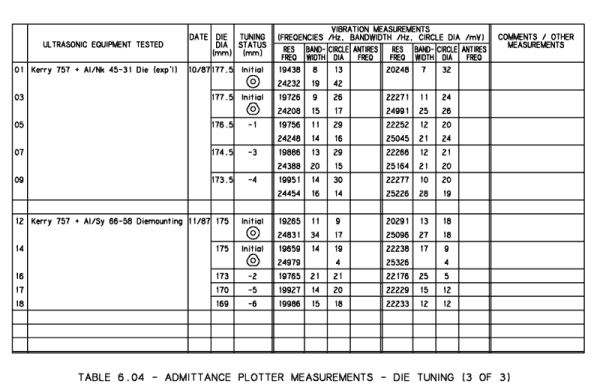
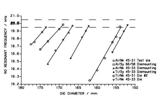
Figure 6.05 - Frequency increase during die tuning
When the die was retested the change in measured performance was dramatic, as shown by the results of item 3. The separation between the R0 and R3 frequencies has been increased from 0.8 to 2.5 kHz, and at the same time the size of the R0 circle has increased while the R3 circle has shrunk. The prime aim of using the shaped die was to increase the frequency separation but both of these effects act to reduce the chances of mode-switching.
Remember, however that there is a price to be paid for this improvement in the frequency performance of the die. The axisymmetric (R0) mode becomes distorted as if by addition of some R3 mode, causing a variation in the vibration amplitude around the die. This is described in more detail in section 3.6.
The subsequent tuning of the die was accomplished as normal but some differences from the tuning of round dies were noted. The rate of increase of the R0 frequency as the diameter was reduced is less than normal (see figure 6.05). This would be expected because when machining down a shaped die less material is removed than from a round die (the flatted areas are not touched). Also the R3 frequency did not change significantly during the tuning process (ie the rate of increase of the R3 frequency is effectively zero). Finally note that the tuned outside diameter is greater than that predicted earlier for the round die. Extra material is needed between the flats to make up for what is lost.
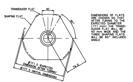
Figure 6.06 - Example of 3-flat shaped die design
The die described above was made as a test of the shaped die concept. For that application other material combinations were known which would give perfectly satisfactory results using the simple round die. There are other applications, however, for which no combination of the known materials would be satisfactory without using a shaped die. This is described in section 4.5.3. One such application is the necking of 66 mm beverage cans to 58 mm diameter. For this purpose a diemounting (combined die and mounting) was constructed using an aluminium outer die with a syalon insert. This was the first real application of the three-flat concept.
The results for this diemounting are listed in table 6.04, items 12 to 18. Again measurements were taken before and after machining the three flats, and during subsequent tuning by reducing the outside diameter. Again the flats were specified with the aim of achieving a 60° included angle after tuning. The distance from the centre to each flat is 73 mm, giving a theoretical 60° included angle at 168.6 mm diameter. The tuned diameter of 169 mm gives an included angle of 60.5°. The listed results for this die are almost identical to those of the experimental three-flat die described above. The final measured performance (based on circle diameter and frequency separation) is perfectly satisfactory.
6.2.2.3 Admittance plotter measurements - dies and mountings
Table 6.05 shows miscellaneous measurements made on a wide variety of ultrasonic dies from all stages of the project. In this section their characteristics and performance will be compared.
Items 1 and 2 are measurements of a solid aluminium test die, taken first with the die placed on the bench on edge, and second with the die suspended by a piece of string through its centre. Comparing these measurements shows no significant change in the resonant and antiresonant frequencies but a significantly smaller circle for the die placed on edge and a correspondingly
larger half-power bandwidth. These two cases tend to represent the extremes of fixing losses - for dies placed on one face (the usual method of testing) a circle diameter somewhere in between would be expected.
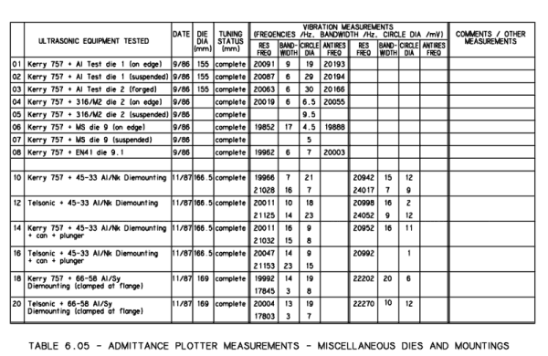
Items 2 and 3 can be used to compare the test die (number 1) with another (test die 2) which was manufactured from a billet of aluminium which had been forged to give a grain structure which was expected to be more favourable to the radial vibrations. The forging was done by taking a 5 inch diameter bar of aluminium alloy and forging it axially to half its original length, causing the diameter to grow to about 7 to 8 inches. The same grade of aluminium was used for both dies and they were geometrically identical. Comparing items 2 and 3 it is clear that there is no significant difference between the measurements made of these two dies. It is possible that the modified grain structure of the forged die could make it more fatigue-resistant but this could not be verified without testing to destruction at high amplitude (which was not done).
Items 4 and 5 again show a comparison of measurements made with the die on edge and suspended. The die in this case is one of the early design dies intended for necking a 45 mm aerosol can to 25 mm diameter (this process was never successful). The die was constructed using an M2 insert in a stainless steel (316) outer. Neither of these materials has been commonly used in more recent dies, the M2 because alternatives are available which are harder or more convenient to use (see section 3.6) and the 316 because it is far more lossy than the preferred titanium and aluminium alloys. This is shown by the admittance circles which are less than half the size of those of comparable dies made in the preferred materials. Again a smaller circle results from placing the die on edge while taking the measurements.
Items 6, 7 and 8 are the results for two more early dies used for necking the 45 mm aerosol to 33 mm diameter. For a quick, cheap trial the first die was made from solid mild steel (die 9) and a duplicate was subsequently made in EN41 tool steel (die 9.1). The small circle diameters (5 to 7 mV) indicate heavy losses, particularly for the mild steel die.
It is interesting to compare the circle diameters measured for these early dies with the circle diameter of the transducer system which was used at the time (table 6.01 item 12, discussed in section 6.2.2.1). Neglecting losses in the piezo-electric transducer (reasonable considering its much larger circle size) it can be said that the losses in the magnetostrictive transducer system are approximately three times greater than in the worst die (based on the ratio of circle diameters). This would indicate that the early dies were in fact perfectly adequate in that system. The need for more efficient dies only becomes apparent when an efficient piezo-electric transducer is used.
Items 10 to 16 show some measurements of the aluminium / ferro-titanit die for necking 45 mm aerosols to 33 mm diameter. The poor performance of this die (ie the closeness of the unwanted R3 frequency) has been discussed previously. In this series of tests the die was
installed in the forming rig using an aluminium tuned mounting. It was not possible to measure admittance while forming a can (the necking process is too fast) but to simulate the type of loading this would impose on the die a fully formed can was pushed into the die and held there by the internal forming tool (plunger). Pressurized air in the pneumatic cylinder which operated the plunger ensured that a constant force (approx 3 kN) was applied to clamp the can into the die. Two types of transducer (Telsonic and Kerry) were also tested. The aim of these measurements was to gain a better understanding of the problem of mode switching (particularly for this die) and why the Telsonic system did not seem to suffer from it.
Without the can and plunger loading the die the results are mostly similar for the two transducers. In each case the R0 circles (at approx 20.0 kHz) are satisfactory, and two unwanted frequencies appear, close together at approx 21.0 kHz. Another harmonic frequency appears at 24.0 kHz in both cases. The interesting feature here is the pair of harmonic frequencies at 21 kHz. Analysis predicts only the R3 near this frequency, but in general a pair of resonant frequencies could be expected for every non-axisymmetric resonance. One of the resonant frequencies would correspond to the R3 mode aligned with an antinode at the transducer, and the other aligned with a node at the transducer.
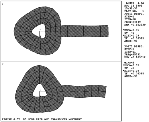
Normally the first mode should be driven by the transducer and the second one filtered out because the die motion will not match that of the transducer. This effect is also discussed in section 2.4.1 The only significant difference between the results for the two transducers concerns the relative sizes of the circles for the pair of R3 frequencies. For the Telsonic transducer the lower frequency resonance has a very small circle diameter (2 mV) but using the Kerry transducer both circles are relatively large (12 and 7 mV). This indicates that the transducer is vibrating unevenly, at least for some of the time, and this may have contributed to the mode-switching problem. Figure 6.07 shows (much exaggerated) how the two modes could look and the sort of uneven motion the transducer would need in order to excite them.
Comparing the results for the die with the can and plunger inside it the two transducers again give very similar results, again with the exception of the relative sizes of the two R3 frequencies. Using the Telsonic transducer one of the R3 pair is large (15 mV) while the other is small (1 mV), but using the Kerry transducer the two circles are again of similar size (11 and 8 mV).
Comparing results for the die loaded (by the can and plunger) and unloaded the following observations can be made: The circle diameter for the R0 mode is reduced when the die is loaded.
The circle diameters for the R3 mode pair are not much reduced, particularly for the Kerry transducer.
The R0 resonant frequency is increased by about 40 Hz when the die is loaded.
The resonant frequencies of the R3 pair are not increased much (on average 10 Hz) when the die is loaded.
All of these effects will, in general, tend to promote mode switching by bringing the unwanted resonances closer to the working frequency and increasing the size of the unwanted resonance relative to the R0. The magnitude of the changes is small in proportion to the relatively small amount of loading applied by the plunger (compared to the necking process). Nevertheless trends are apparent which must tend to destabilize the R0 mode, and the Kerry ultrasonics system is measurably less stable than the Telsonic. Whether mode switching takes place will depend not only on the stability of the transducer and die (as indicated by these measurements) but also on the quality and stability of the control system used to maintain resonance. The fact that mode switching has been observed in this die using the Kerry system indicates that for this equipment the limit has been reached. For the Telsonic equipment (which probably also employs a superior control system) the limit has not yet been found.
Finally, items 18 and 20 of table 6.05 show measurements of the aluminium diemounting with syalon insert for necking 66 mm beverage cans to 58 mm diameter. The tuning of this die was described in the previous section (items 12 to 18 of table 6.04). These measurements differ only in that the diemounting was clamped by its flange. Comparing these measurements with the final tuning measurement shows no significant differences, indicating that clamping the flange has minimal effect on the die vibrations. Comparing the results for the two transducers shows no major differences.
6.2.2.4 Admittance plotter measurements - mounting evaluation
Tables 6.12 and 6.13 show evaluations of the performance of a number of tubular tuned mountings. These are discussed in section 6.4.
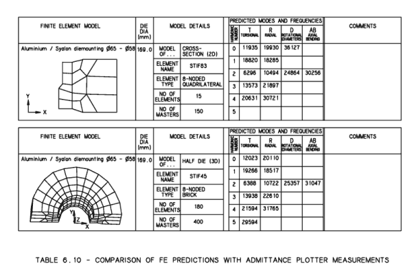
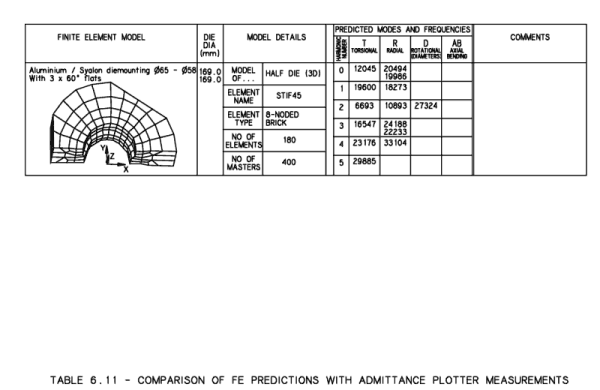
6.2.3 Comparison with FE predictions
For the results shown in tables 6.02 to 6.04 (the die tuning operations) corresponding information from the finite element analysis has been summarized in tables 6.06 to 6.11 to give an indication of the normal levels of accuracy. In each case the type of finite element model and the number of elements and master degrees of freedom is indicated, followed by the predicted natural frequencies (for the die alone) categorized by the system of mode nomenclature described in section 3.1. The actual outside diameter and measured frequencies (as also shown in tables 6.02 to 6.04) have also been included in heavy type. Note that for some models (the round versions of the three-flat dies) no real measurements have been included because no equivalent die was produced.
Tables 6.06 and 6.07 show the analysis of conventional (round) dies. This type of analysis is straightforward and efficient using two-dimensional axi-symmetric harmonic elements (see section 2.4.3 for a full description of this type of element). The number of elements ranges from 52 to 62 and the number of masters from 100 to 130. Comparing the predicted and actual results shows that the predictions were generally good, with the maximum difference on diameter only 1.3 mm and the agreement on R0 and R1 frequencies well within 1%.
The only significant error is the consistent overestimating of the R3 frequency (by about 0.5 to 1 kHz, or 2.5 to 5%). There are two sources of error contributing to this. Firstly the tendency of the FE model to overestimate the frequencies, particularly of the harmonic modes (as discussed in detail in section 2.8). Secondly the finite element model does not include the transducer, whereas all measurements inevitably do. The effect of the transducer is to "pull" frequencies towards its own working frequency, 20 kHz. These two sources of error will tend to cancel out for frequencies below 20 kHz (typically the R1 frequencies) but will add together for frequencies above 20 kHz (ie the R3).
Tables 6.08 to 6.11 show the results for the FE models of the two 3-flat designs (for which the measured results are shown in table 6.04). Modelling this type of die is more difficult because the axi-symmetric elements are no longer applicable. A similar analysis of the die using a full three-dimensional model was required but limitations on the computing power available made this impossible to analyse. As a compromise a simpler 3-D model with a coarse mesh was analysed and the results compared with 2-D axi-symmetric models.
The results of this analysis for the experimental Aluminium / Nikro die are shown in tables 6.08 and 6.09. Table 6.08 (top) shows the axi-symmetric model similar to those used for the four round dies described previously. In this case the predicted R3 frequency was 21.2 kHz (lower than any previous die). This is well within the "danger zone" around 20 kHz and it is likely that the actual frequency would have been even lower, for the reasons described above. This was confirmation that the 3-flat design was required.
Table 6.08 (bottom) shows the results for the same model and the same axi-symmetric elements but with a much coarser mesh (only 18 elements compared to the 62 used earlier). This was done because it was known that a coarser model would be needed for the 3-D analysis and the coarse mesh 2-D model would provide a better comparison. Comparing the results for the two 2-D models shows that all the coarse model frequencies were higher (less accurate), and the largest discrepancies were in the torsional mode frequencies and the higher harmonic radial modes. The predicted R3 frequency was increased by 0.5 kHz in the coarse model, indicating the necessity of a reasonably fine mesh.
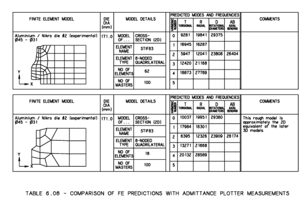
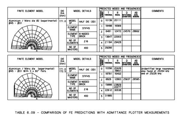
Table 6.09 (top) shows the results for the 3-D model round die. This was equivalent to the two axi-symmetric models and permitted a further comparison of probable accuracy of the different models. The predicted frequencies for the 3-D model were all higher again (even less accurate) than those of the coarse 2-D model and in this case the predicted R3 frequency was 22 kHz which, if true, would have been acceptable.
Table 6.09 (bottom) shows the results for the 3-D model 3-flat die. Knowing the inaccuracy of these models, these results were treated with caution, but comparison with the round die model was expected to indicate the true results. Comparing the most important (for this die) R0 and R3 frequencies, the effect of the 3-flat design is to raise the R0 slightly (by 0.3 kHz) and to raise the R3 considerably (by 1.8 kHz). This indicated that the separation between R0 and R3 frequencies should be increased by 1.5 kHz.
The measured results for this die are also shown in table 6.09 (bottom). Comparing these, the predicted die diameter is 2.5 mm less than the actual (not enough allowance was made for the flats increasing the R0 frequency) and the R3 frequency was, as expected, greatly overestimated (by 1.6 kHz). The most important point to note, however, is that the R3 frequency, at 22.3 kHz, was fully acceptable. The 3-flat design had increased the frequency separation as predicted.
A similar procedure was used for the design of a die for necking 66 mm beverage cans to 58 mm diameter. As discussed in section 3.7, choosing alternative materials for the construction of this die did not produce any results which would be acceptable. The use of a shaped die was therefore essential, and the predicted natural frequencies indicated that the (3-flat) design would be suitable. The results in tables 6.10 and 6.11 are for three models, one 2-D axi-symmetric (coarse mesh), one 3-D round and one 3-D with flats. As before the frequencies are significantly overestimated by the 3-D models but increased separation between R0 and R3 frequencies is achieved, much as predicted. During tuning the die diameter was machined to exactly the size predicted (169 mm) and the measured R3 frequency was then found to be 22.2 kHz - fully acceptable.
6.2.4 Accuracy of FE predictions
The potential accuracy of the FE models is discussed in section 2.8, but comparison with real measurements (as described here) introduces some further sources of error:
1) Tolerances on dimensions and variations in material properties may result in the die failing to match its finite element model perfectly.
2) The presence of a transducer on the die during frequency measurements will itself affect the resonant frequencies.
From the results described in the previous section it appears that these sources of error can account for up to about 3 mm discrepancy in the tuned outside diameter of a typical die. To allow for this the dies are initially manufactured about 6 mm oversize and then tuned by gradual machining down. The 6 mm "tuning allowance" could be reduced but there is little advantage in doing this because the dies are usually manufactured by turning down a stock size bar (eg 7" diameter).
The two-dimensional axi-symmetric harmonic elements offer good accuracy and efficiency.
To analyse the shaped dies only a full three-dimensional model is suitable, but limitations on available computing power required the use of a much coarser mesh for this type of model which was far less accurate. The technique adopted, using both 2-D and 3-D models gave satisfactory results.
Harmonic frequencies above 20 kHz tend to be overestimated by the FE model, while harmonic frequencies below 20 kHz are generally reasonably accurate.
6.3 ESPI MEASUREMENTS
One of the most powerful techniques used to evaluate the performance of ultrasonic dies was Electronic Speckle Pattern Interferometry (ESPI). The technique was developed for use on ultrasonic dies by Tyrer and Shellabear [117], [118], [119], [120] along with others at Loughborough University during the course of the SERC-sponsored project. This non-contact measuring system was capable of giving quantitative data for the vibrations of the whole die in real time.
There are however some disadvantages of this system compared to the other systems described previously, particularly the cost and setting up time. Another potential problem is the interpretation of the results produced by ESPI which are not always immediately understandable. To assist in identifying modes of vibration it was necessary to process the finite element results to produce an image equivalent to an ESPI picture.
This section describes the general principles of ESPI and the techniques used to interpret the results by comparison with finite element models.
6.3.1 Principles of ESPI
For a full explanation of the technique see the various publications of Shellabear, Tyrer et al [117], [118], [119], [120]. The die is illuminated by an interfering pair of laser beams, producing a speckle pattern. A video camera is used to digitally record an image of this pattern. Any movement of the die surface causes changes in the speckles, depending on the distance moved. By digitally subtracting the new image from the previous stored one, the changes are shown, with light and dark fringes showing areas where the amount of movement is similar (like contour mapping). By different arrangements of the laser beams the equipment can be made sensitive to movements along three orthogonal axes (ie with the die set up on a horizontal axis, movements can be measured out-of-plane, in-plane horizontal and in-plane vertical).
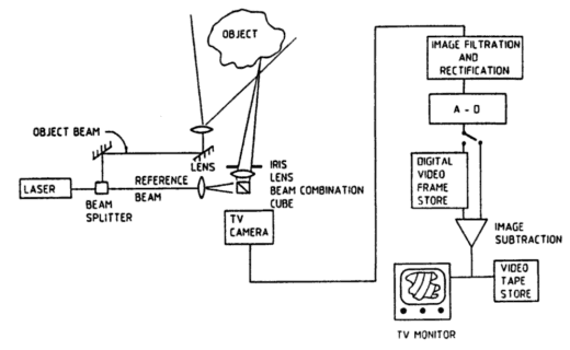
Figure 6.08 - ESPI General Arrangement
For identifying pure modes of vibration the out-of plane image is useful because in most cases the axial motion gives a good idea of the nature of the mode (ie its harmonic number and whether it is predominantly radial or torsional). However it does not show directly the most useful component of vibration (the radial component), and where there is a mixture of two modes one (with predominantly radial motion) may be masked by the other (with significant axial motion).
The two in-plane images will provide the extra information required but they are much more difficult to interpret because they show elements of both radial and hoop motion in different areas of the die. If amplitude and phase information is known then the precise motion of the die at any point can be evaluated from the three images (and Shellabear [120] has done this) but the process is laborious and often the full set of results is not available. The alternative chosen for much of this work was to process the finite element results for each mode into simulated ESPI images which could be compared with the real ESPI images as they were generated.
When this was done it was found that some images matched well but others seemed to contain elements of the FE images for more than one mode of vibration. It is to be expected that the modes of vibration of a real die, in the presence of imperfections and damping, will not be pure but in general will be combination modes made up of a number of pure modes.
To allow for this in the interpretation of the ESPI results a program was produced to process the FE results, not only converting them to ESPI type images but also allowing the combination of a number of different (pure) modes in proportions chosen by the user. Thus using the program and selecting mode combinations by trial-and-error the user could find a combination which produced a set of images to match the real ESPI results. While not positive proof of the nature of the vibrations of the real die this gives a very good indication.
6.3.2 Converting FE results to simulated ESPI plots
6.3.2.1 Pure modes
The Ansys program produces a huge amount of data for even the simplest model. To avoid wasting processing time and storage the relevant finite element data was first extracted and stored in a series of data files. Each file included a set of data (the radius and three components of displacement) for all nodes along a radial line on one face. The data for each mode was stored in a separate file.
Note that a 2-D axisymmetric-harmonic finite element model was used (section 2.4.3). A 3-D model could have been used but the 2-D model is more efficient. The variation in the components of amplitude over the surface of the die can be accurately predicted using the known harmonic variation as described in section 2.4.3 (the harmonic number is also stored on the data file).
The main program was written in Fortran using the Issco Codebook prototype [123]. This is a program which takes the user through a question and answer session and then automatically generates the Fortran source code to produce the required plots by calling subroutines in the "Disspla" library. The technique is similar to that of example 3.6.6 (appendix 3) for making contour plots of the performance of different die designs. After the plotting program is generated it can be edited to perform other functions (in this case data processing) and recompiled like any other program. The final result is a program which is less tidy than one written specifically for the application but which takes less effort to produce.
To display a pure mode the program must read in the data for that mode from the appropriate data file and then use the data to calculate the component of amplitude in a chosen direction (axial, horizontal or vertical) at points all over the die face. The result is stored in a 2 x 2 array and subsequently displayed using colours corresponding to the light and dark fringes produced by ESPI.
The calculations must take into account:
1) The radial and angular position of the point.
2) The harmonic number.
3) For horizontal and vertical components: both radial and hoop amplitudes.
4) For harmonic number greater than 0: The angular alignment of hoop components of amplitude (hoop amplitude is zero at the radial / axial antinode).
6.3.2.2 Distorted modes
For distorted modes (ie combinations of two or more pure modes) the procedure is the same but the components of amplitude for each mode must be added together.
The program in its latest form allowed the user to select one main mode and one secondary mode. The reference angle for each one can be specified (ie where on the image the mode's antinodes should appear) and for the secondary mode the fraction of that mode which should be added. Future enhancements may include the option to add a third mode if this becomes necessary.
6.3.3 Comparison of results
Figures 6.09 to 6.13 show typical ESPI-equivalent images generated from the finite element data and actual ESPI photos from Shellabear's work. The computer-generated images correspond to the pure modes which are generally of interest, because they typically appear at a frequency close to 20 kHz. The photos (where available) show the closest measured response modes of the die.
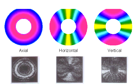
Figure 6.09 - ESPI images (predicted and actual) - R0 mode
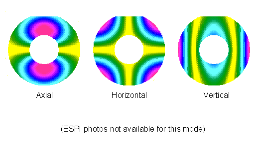
Figure 6.10 - ESPI images (predicted) - R1 mode
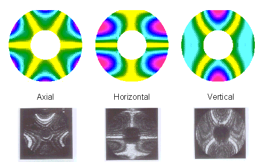
Figure 6.11 - ESPI images (predicted and actual) - R3 mode
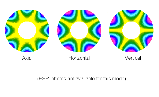
Figure 6.12 - ESPI images (predicted) - T4 mode
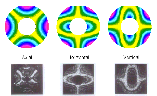
Figure 6.13 - ESPI images (predicted and actual) - D2 mode
These results have been produced for an aerosol necking die comprising a ferro-titanit insert in an aluminium outer (die materials are discussed in section 3.6). Other die designs produce ESPI-equivalent images which are generally similar.
Photos taken from the ESPI video pictures are shown in references 1 (for R0, R3 and D2 modes) and reproduced here, where available, along with the corresponding simulated ESPI image. This allows easy comparison of the theoretical vibrations with the real measurements.
For the R0 and D2 modes (figures 6.09 and 6.13) the correlation with the pure mode FE results is clear, although some vertical distortion of the fringes is apparent. This is to be expected particularly for the D2 mode because the frequency (24 kHz) is significantly separated from the 20 kHz working frequency. This means that the transducer unit which drives the die must be detuned and therefore effectively applies a mass to the outside of the die moving in a vertical direction. Nevertheless the images match well enough to clearly identify both modes.
For the (presumed) R3 mode (figure 6.11) the correlation is less clear. It was believed to be a distorted R3 mode because its natural frequency (20.8 kHz) approximately matched the FE prediction and because the image for axial motion shows a three-way symmetry (although for the pure R3 mode a six-way symmetrical image would have been expected). The closest other mode to this one is the R0 at 20 kHz so it was expected that the distortion would take this form. Figures 6.14 to 6.16 show different combinations of R3 and R0 modes. In figure 6.14 the R0 mode at half-amplitude has been added, but this shows a distortion opposite to that shown by the real measurements. Figure 6.15 shows the R0 mode at half amplitude subtracted from the R3, and this shows good agreement with the measurements. Note that for each mode the amplitude is normalized but the sign is purely arbitrary. Figure 6.16, shows the combination R3 - 0.2 x R0. Judging by eye, the best correlation is probably somewhere between the last two, ie. R3 - 20 to 50% R0.
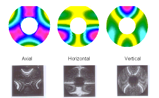
Figure 6.14 - ESPI images - Combination R3 + 0.5 R0 mode
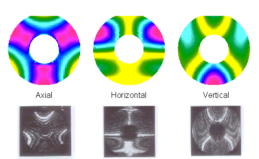
Figure 6.15 - ESPI images - Combination R3 - 0.5 R0 mode
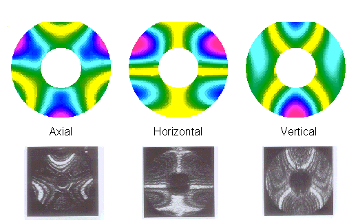
Figure 6.16 - ESPI images - Combination R3 - 0.2 R0 mode
6.3.4 ESPI Summary
A method of processing finite element results has been demonstrated which produces images equivalent to those of the real die produced using electronic speckle pattern interferometry (ESPI).
When used for comparison with the images of a vibrating die these simulated ESPI images allow interpretation of the mode of vibration.
For cases where the mode of vibration is not a pure mode its composition may be evaluated by comparison with an image produced for two pure modes combined in a specified ratio.
6.4 EVALUATION OF TUBULAR MOUNTING PERFORMANCE
Between the initial concept for the thin walled tubular mounting (described in chapter 5) and the final optimized design, several attempts were made to measure its performance. These will be described in turn.
6.4.1 Free vibrations of steel prototype
The first prototype was manufactured in mild steel (for minimum cost). This was a tube of inside diameter 80 mm, outside diameter 85 mm and length 130 mm with a central flange as shown in figure 6.17. This corresponds to the initial concept of a tube resonant simultaneously in both radial and longitudinal modes. Finite element analysis predicted a large number of free vibration modes in the region of 20 kHz. An experiment was planned to measure these frequencies.
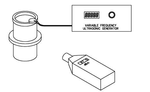
Figure 6.17 - Testing free resonances of tubular mounting
In order to excite vibrations in the die while it was not connected to the die a small piezo-ceramic disk was fixed (using epoxy adhesive) to the free end of the mounting. This was driven electrically by a small variable frequency generator. Motion of the tube walls was sensed by a noise level meter mounted at a fixed distance from the mounting. Thus sensing was entirely non-contact but driving the vibrations involved the addition of a small mass to the system which would inevitably affect the frequencies. The effect was minimal, however, because of the small volume and relatively low density of the piezo-ceramic disk compared to the steel tube.
The measured results are shown in figure 6.18. The points on the resonance curve have mostly been confined to resonances (peaks) and antiresonances (troughs) because of the huge number of resonances involved. Identification of the modeshapes was not possible because of the method of measurement, but the nature of the resonance curve was generally as predicted (ie many resonances around 20 kHz).
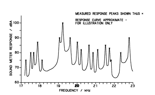
Figure 6.18 - Resonant frequencies of steel tubular mounting
Indeed the number of measured resonances would have been doubled relative to the axi-harmonic FE model because the piezo-ceramic disk would slightly "unbalance" the tube creating a pair of resonances for each of the theoretical ones.
Further trials on the free mounting were not expected to yield any more useful results so all subsequent testing was done on the combined system (die and mounting).
6.4.2 Admittance plotter measurements of mounting performance
The admittance plotter (described in section 6.1.2) gives an accurate and sensitive measure of the characteristics of a mechanical system comprising a transducer and other components connected to it. In order to evaluate the effect of the mounting it was necessary to compare the transducer, die and mounting against the transducer and die alone. The results of this and some other comparisons for several dies and mountings are recorded in tables 6.12 and 6.13, and will now be discussed in turn.
All the measurements listed in table 6.12 are for the aluminium test dies with various early mountings fitted. Other measurements on these dies (section 6.2.2.3 and table 6.05) showed that the dies were effectively identical and that circle diameters for either die with a Kerry transducer would range from 19 to 30 mV depending on the position of the die (resting on the bench or hanging on a string etc).
Items 1 to 4 show some measurements of the test die fitted with the first aluminium mounting. This was dimensionally identical to the steel mounting (ie not optimized) and fitted to the back of the die by screws through a flange (figure 6.19). The measured circle diameters are significantly less than for the die alone, and the smallest circle (10 mV) was measured with the mounting flange clamped in place. This indicates that power losses from this system would be high.
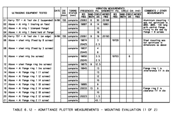
Items 5 to 10 show measurements of the other test die with the first steel mounting fitted. These show two problems. Firstly there were three measurable resonances around 20 kHz - this means that the mass of the mounting is great enough for its own resonances to seriously influence the whole system (particularly because the die is aluminium and hence relatively light). Secondly the circle diameters are all very small (at best only half of the smallest circle for the aluminium mounting). The three measurements were made to estimate the effect of the fixing screws. There was no significant difference when using eight, three or no screws.
Items 12 to 21 take these experiments further with three rings (one steel and two aluminium) which fitted into the back of the die in the same way as the mounting. All measurements were made with the die on its edge for direct comparison with item 5. When the steel ring was fitted (without screws but using an interference fit) there were significant additional losses (circle diameter reduced from 19 to 12.5 mV). Similar results were obtained for the first aluminium ring, which was also an interference fit in the die. In this case the fixing screws were also used and the circle plotted for one, two, four and all eight screws inserted. With the screws inserted both the resonant frequency and the circle diameter decreased indicating that the screws were adding both extra mass and extra losses. The second aluminium ring was a clearance fit in the back of the die. When this was fixed by four or eight screws its results were identical to those of the first aluminium ring, but when it was held by only two screws (fitted on opposite sides) the circle diameter became very small (1.5 mV) and held by only one screw the resonance was effectively eliminated.
This series of trials demonstrated that the mounting flange screwed to the back of the die was generally undesirable. The simple interference fit was better but even this was not ideal. For later dies and mountings the fixing system was redesigned as shown in figure 6.19. The flange and fixing screws were eliminated in favour of a simple interference fit. Furthermore the end of the mounting tube was increased in thickness to increase its rigidity (and so improve the effectiveness of the interference fit) and at the same time maintain the 20 kHz resonance which had been lost when using the flange. After design optimization the interface was eliminated altogether by manufacturing the die outer and the mounting together in one piece.
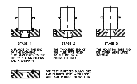 Figure 6.19 - Fixing of tubular mounting to the die
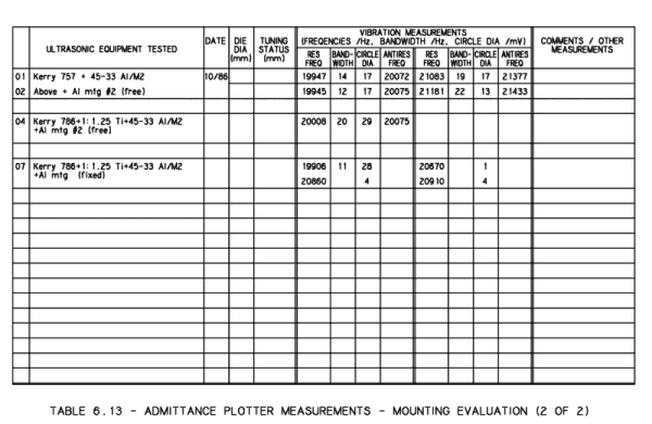
Table 6.13 shows some further admittance plotter measurements used for evaluation of tubular mountings. Items 1 and 2 are results of circle plots for a die with and without an aluminium mounting fixed by interference fit only. The results show that the effect of the mounting is minimal. Items 4 and 7 (for the same die and mounting, but using a different transducer and a booster) show that the mounting flange can be fixed with minimal effect on the die performance.
Subsequent mountings were made integral with the die, to eliminate potential losses at the interface. Some of these were described in sections 6.2.2.2 (die tuning) and 6.2.2.3 (miscellaneous dies and mountings). The good measured performance of these "diemountings" in comparison with the earlier dies is evidence for the success of the design.
6.4.3 Tubular mounting measurements - summary
These results show that in general the mounting has little effect on the resonant frequency of the system (presumably it is dominated by the greater momentum of the die) but adds some power losses to those of the remainder of the system. Additional losses for early designs running at 20 kHz, 10 μ amplitude were approx 300 W. Later versions under the same circumstances would use less power (of the order 100 W) but this was difficult to evaluate because in these later dies the mounting was made integral with the die outer (no shrink fit) so direct comparison with and without mounting was not practical.
This type of mounting (particularly in the later versions with optimised geometry) has therefore been shown to be a practical and efficient method of mounting the ultrasonic die.
6.5 MEASURED PROCESS FORCES
The process of necking welded cans (ie reducing the diameter of one end) is discussed in detail in section 1.1, along with the various problems which can occur. In this application the prime reason for using ultrasonics is to prevent collapse of the can body. Without ultrasonics the forming force exceeds the strength of the body, which is then crushed as shown in figure 6.20 (as figure 1.09). With ultrasonics the forming force is reduced (for reasons discussed in section 1.2) to less than the collapse force of the can body. The collapse of the can is therefore a crude measure of the process force.
Clearly the crushing / not crushing of the can was not an adequate method of force measurement and a more accurate method was required. In fact two methods of measuring force were used, as follows.
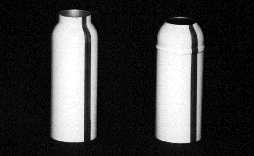
Figure 6.20 - Cans necked successfully and crushed during necking
6.5.1 Evaluation of forming force in early work
In the early part of the project a very simple experiment was conducted. The hydraulic pressure supply to the cylinder used to perform the necking process was reduced so that minimal force would be applied to the can. One can was necked at this pressure and the necking process stopped when the required forming force exceeded the available force (hydraulic pressure x piston area). The neck diameter of the partially necked can was then measured. After a small increase in the supply pressure the process was repeated, and this continued until the available force was sufficient to crush the cans (full forming was not possible at this stage). The result was a set of corresponding forming force and neck diameter data which could be plotted as a graph.
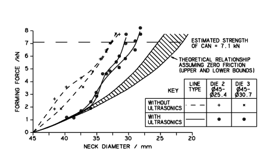
Figure 6.21 - Measured forming force vs diameter (early work)
Figure 6.21 shows the results for cans formed with and without ultrasonics, in dies designed for a final diameter of 31 mm and 25.4 mm. For comparison a graph of the theoretical forming force is also included (calculated using the analysis shown in appendix 1). The analysis takes account of work hardening of the metal (based on measured strength before and after necking) but assumes zero friction. It is remarkable how closely the measured forming force for the cans formed with ultrasonics follows the theoretical curve for the initial part of the forming process (arguably indicating that the process happens with almost zero friction in the early stages). Note that towards the end of the process the measured forces (with ultrasonics) diverge from the theoretical curve but remain significantly lower than the measured forces without ultrasonics. Note also that a smaller diameter was achieved using the 25.4 mm diameter die, almost certainly because extra work is required to bend the material up into the straight section, and because contact with the (non-vibrating) inner tool causes extra friction. This straight section is necessary to provide the material for forming the rolled end ("curl").
6.5.2 Evaluation of forming force in later work
One problem with the method described above is that the can is formed slowly (coming to a complete halt). It has been found that the can is less likely to be crushed if the necking tools move at high speed (there is presumably a limit to this but this was not found within the speed capability of the hydraulic rams - about 0.25 m/s). It was therefore desirable to measure the forming force while the operation proceeded at normal speed. A load cell would have been ideal but this would have been difficult to fit into the forming rig because of various other moving parts. A simpler option was therefore implemented as shown in figure 6.22. Pressure transducers were fitted in the supplies to the hydraulic cylinder which powered the die movement. Two transducers were required to measure pressure above and below the piston.
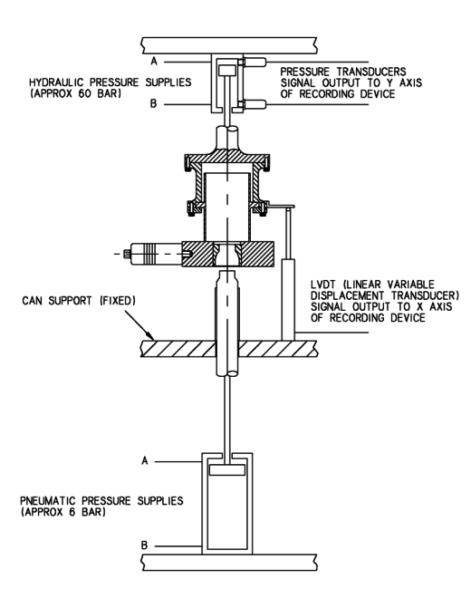
Figure 6.22 - Equipment to measure forming forces on test rig
Forming force was calculated by subtracting (pressure x area) below the piston from (pressure x area) above. An LVDT (linear variable displacement transducer) was also used to monitor the position of the moving die and so provide a reference to the progress of the forming process.
Results are shown in figure 6.23, for cans formed with and without ultrasonics. Note that the can formed without ultrasonics was crushed (causing a sudden drop in the applied force) while with ultrasonics the can was fully formed. The results are transferred to a graph of force vs neck diameter in figure 6.24 and here the graph of the theoretical forming force is also included (as on the earlier force - diameter graph). In this case the measured forming force (with ultrasonics) follows the theoretical curve much further, almost to the end of the forming process. Comparison with the measurements made in the early stages of the project shows that developments in the die technology have led to a further reduction in forming force but that the forming force has not been reduced below the theoretical zero friction force. This is strong circumstantial evidence in favour of the friction reduction theory of force reduction (see section 1.2).
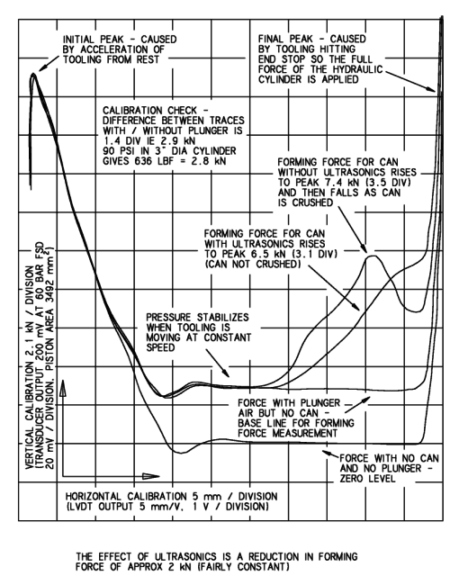
Figure 6.23 - Forming forces measured on test rig with and without ultrasonics
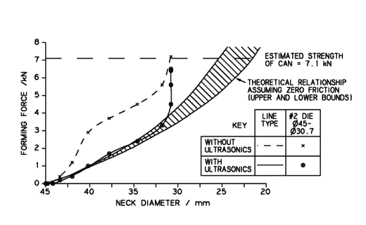
Figure 6.14 - Measured forming force vs diameter (later work)
6.6 CONCLUSIONS
Various methods have been used for evaluation of the die vibrations. ESPI (electronic speckle pattern interferometry) is potentially the most useful, offering full three-dimensional analysis of all visible surfaces of the die, even while forming a can. With further development the disadvantages of this system (cost, setting up and interpretation of results) could be reduced in the future. For evaluation of resonance modes and frequencies the admittance plotter (section 6.2.2) was used most. This gave convenient, accurate and revealing measurements of each die's performance.
Problems of "mode-switching" were found in dies with unwanted resonances close to the working frequency. The use of shaped dies was shown to overcome this problem.
Comparative measurements on dies with and without the tubular tuned mounting showed the improvements obtained by developing the method of attachment and the mounting geometry. The result of this development is a mounting system which accurately locates the die while allowing it to vibrate with minimal loss of energy.
Measurements of the force required to form a can showed that the effect of the ultrasonic vibrations was to reduce forming force by 40 to 60%. Where high reductions are required this may mean the difference between successfully necking the can and crushing it. The reduced forming force corresponded very closely to the theoretical zero-friction force, suggesting that the observed effect of ultrasonics may be caused by reduction or elimination of friction.